3.Seaborn notes
3.Seaborn notes
Seaborn 绘制图形技巧主要在于数据思维难,如:怎么选择字段,怎么选择预处理数据,绘制什么图像,以及要在图像上体现数据统计量及其变化。我们应该去逐一理解数据,选择合适的技巧。下面举例了8个常用的绘制函数。每个函数调用时,针对DataFrame这种数据类型,要注意打算绘制哪些字段(哪些列),用什么绘制函数,输入参数有哪些,主要注意x,y选择的字段。
1.lineplot
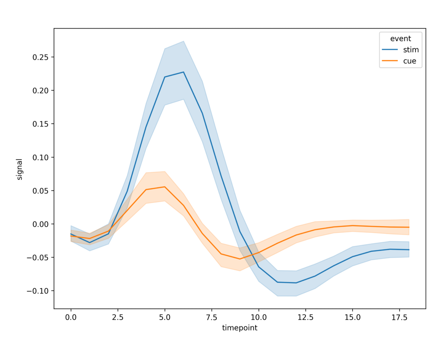
绘制折线图命令:seaborn.lineplot(x, y, data, hue, legend),基本上了解这些参数就可以了。
x,y就是数据的不同列会作为x轴,y轴的输入数据。如果具体指明对应的列,data参数可以不要。如示例中可以改为
sns.lineplot(x=fmri['timepoint'], y=fmri['signal'], hue=fmri['event'])。data可以是df, ndarray等。一般是df,这时上面的x,y参数可以只写列名。hue利用颜色来表示类型变量, 如例子fmri中绘制不同event对应的折线legend图例,默认“auto”。可以选full, 也可以具体制定。如例子fmri右上角event的图例。
拿fmri示例:
1 | fmri = sns.load_dataset("fmri") |
1 | plt.figure(figsize=(8, 6), dpi=300) |
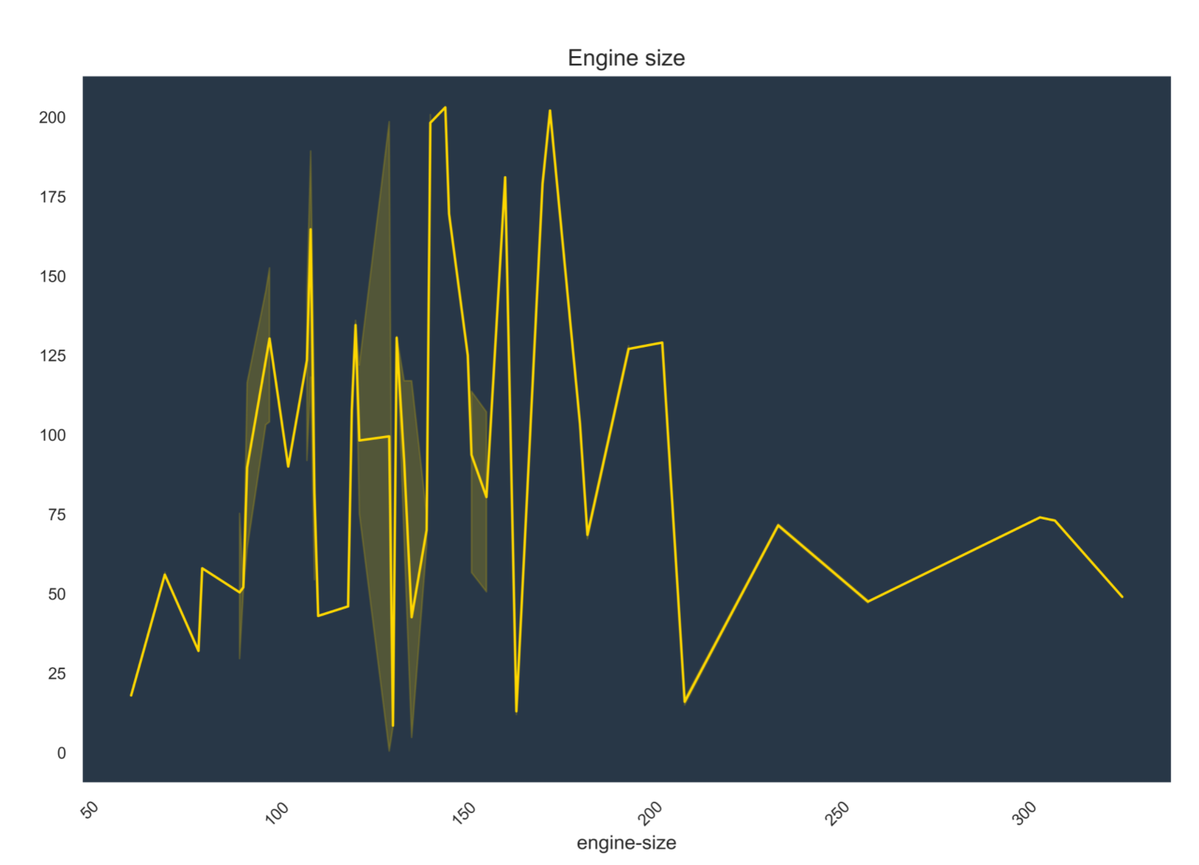
我们来进一步设置,让图更好看一点。
1 | auto = pd.read_csv("Automobile_data.csv") |
auto信息如下:
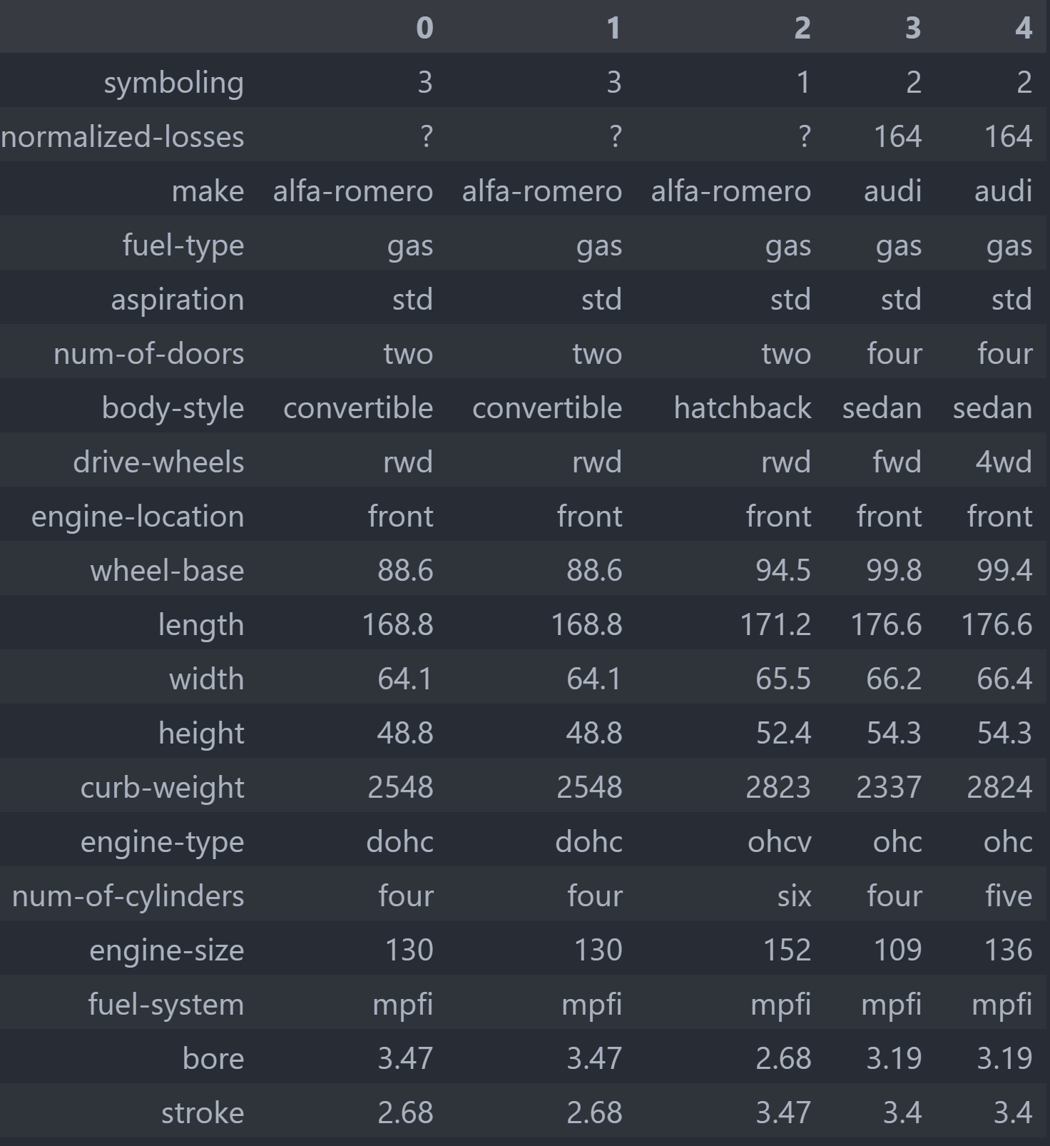
1 | plt.figure(figsize=(12, 8), dpi=500) |
2.Scatterplots
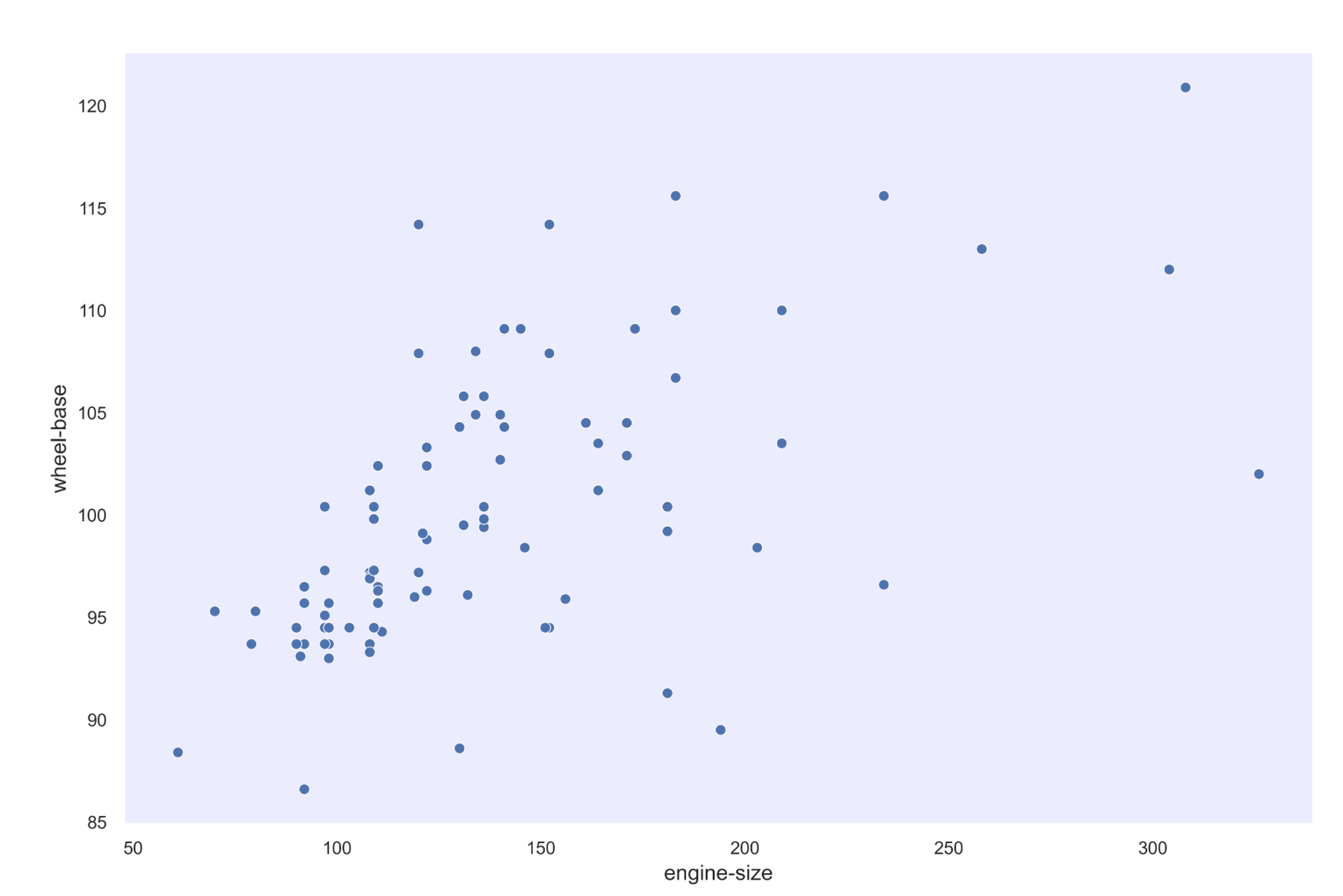
绘制散点图用 sns.scatterplot,其中:
x, y, data用法类似折线图hue用颜色表示类型字段信息。size用点的大小表示类型字段信息。
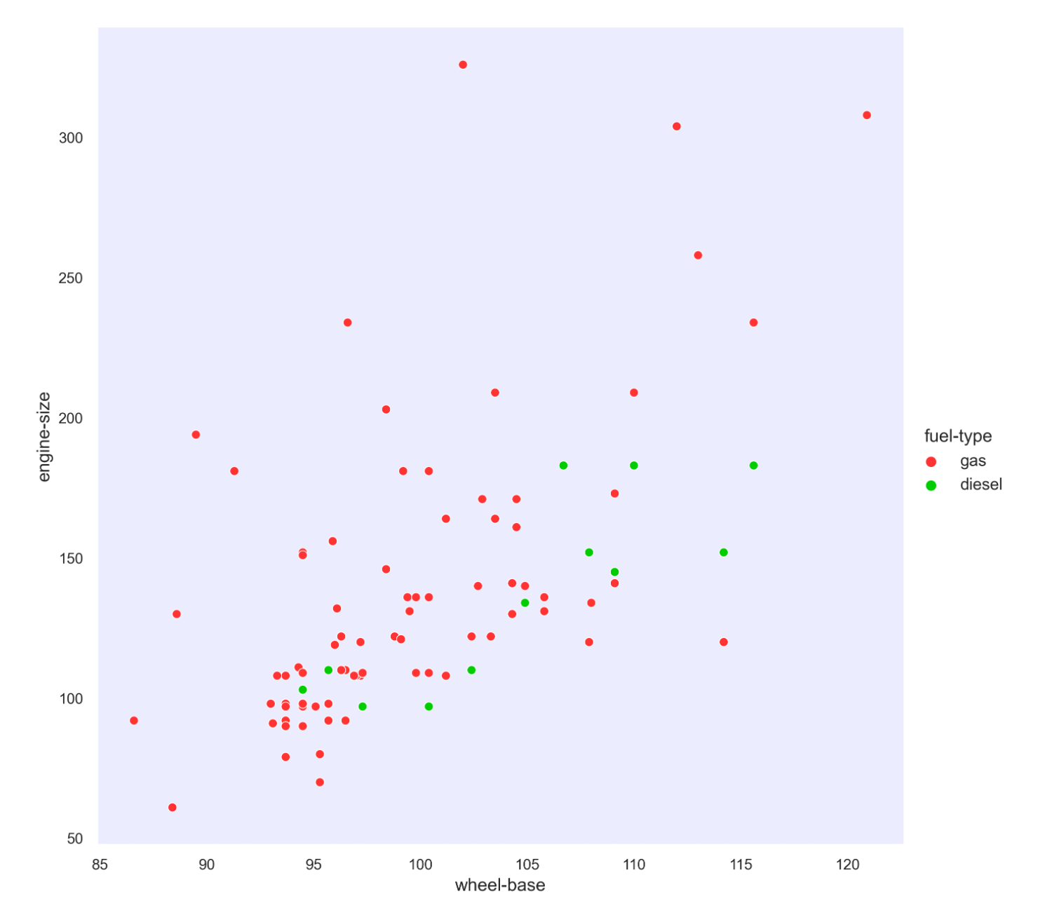
还是 auto = pd.read_csv("Automobile_data.csv")这个df,我们探索 'engine-size'和 'wheel-base'轴距之间的关系。
1 | plt.figure(figsize=(12, 8), dpi=500) |
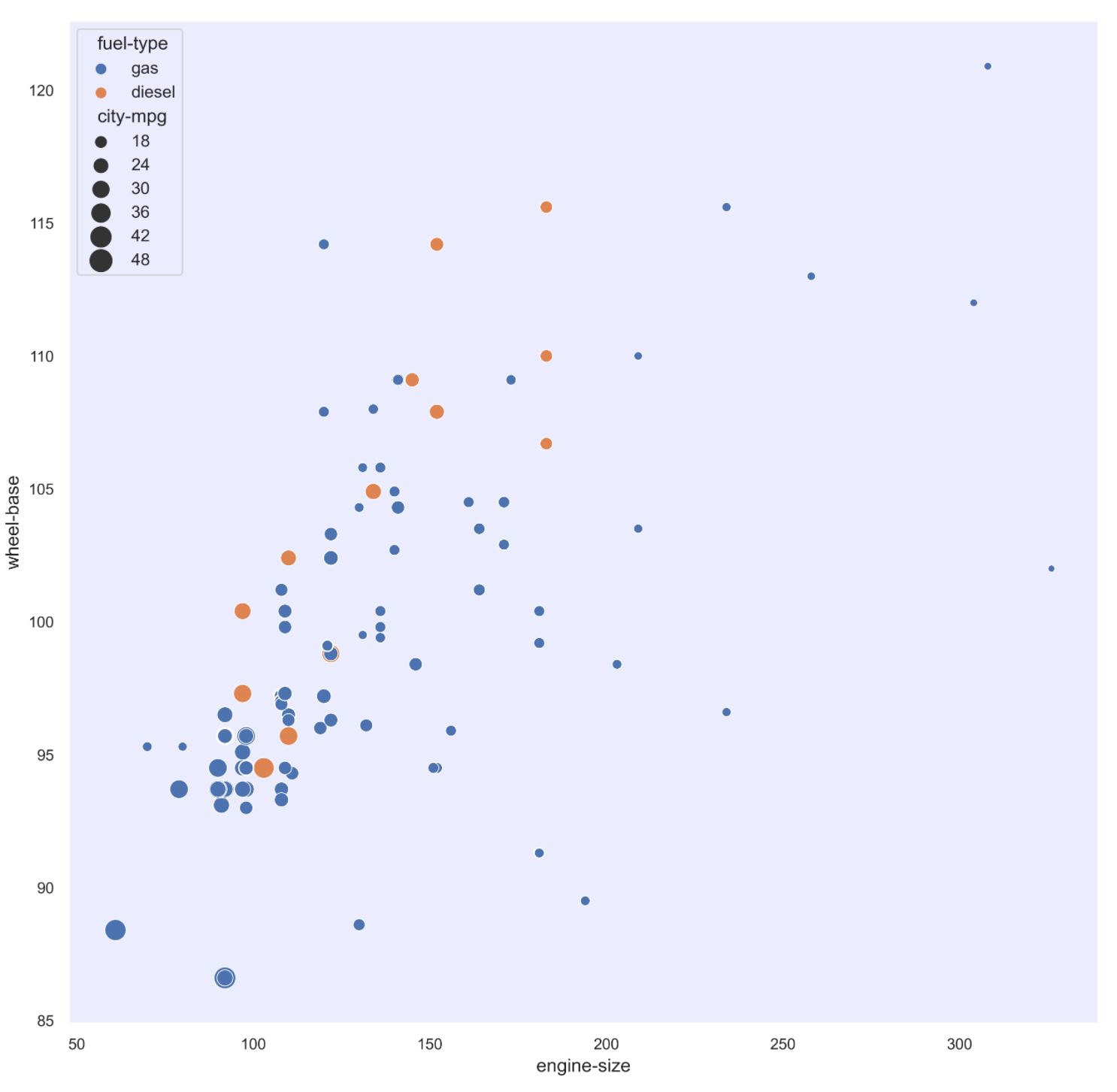
如果我们还要增加 fuel-type字段和 city-mpg字段信息,并只绘制 (20, 200)city-mpg数据,可以用hue颜色表示fuel-type,size大小表示city-mpg。
1 | plt.figure(figsize=(12, 12), dpi=500) |
3. relplot
relplot和scatterplot最主要区别是其有个kind参数可以选择scatter还是line。基本可以看做lineplot,scatterplot合体。
1 | plt.rcParams['savefig.dpi'] = 300 #图片分辨率 |
4.barplot
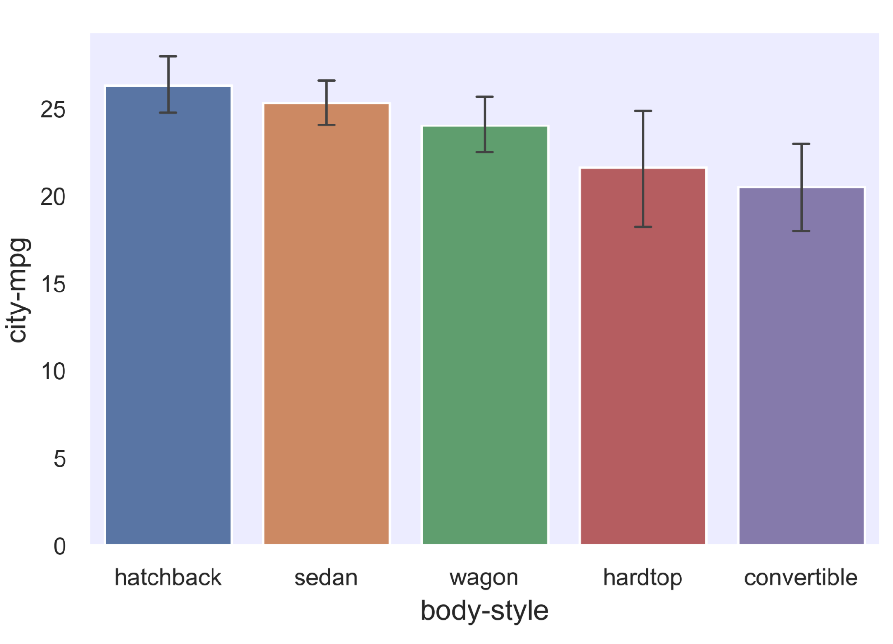
barplot主要绘制数字变量和类别变量关系。示例中的city-mpg和 body-style中的关系。可以将x,y变量调换让其横过来。其中:
order是排序索引capsize指bar的帽子宽度,如示例中两黑色横线。errwidth指bar的线宽。
1 | order = auto.groupby(['body-style']).mean().sort_values(by='city-mpg', ascending=False).index |
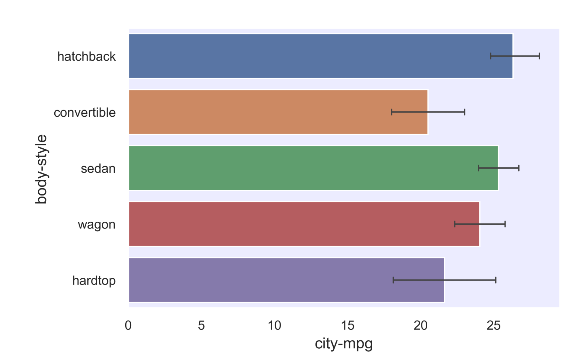
将其x,y调换将图像横过来,并随便指定个顺序。
1 | order = ['hatchback', 'convertible', 'sedan', 'wagon', 'hardtop', ] |
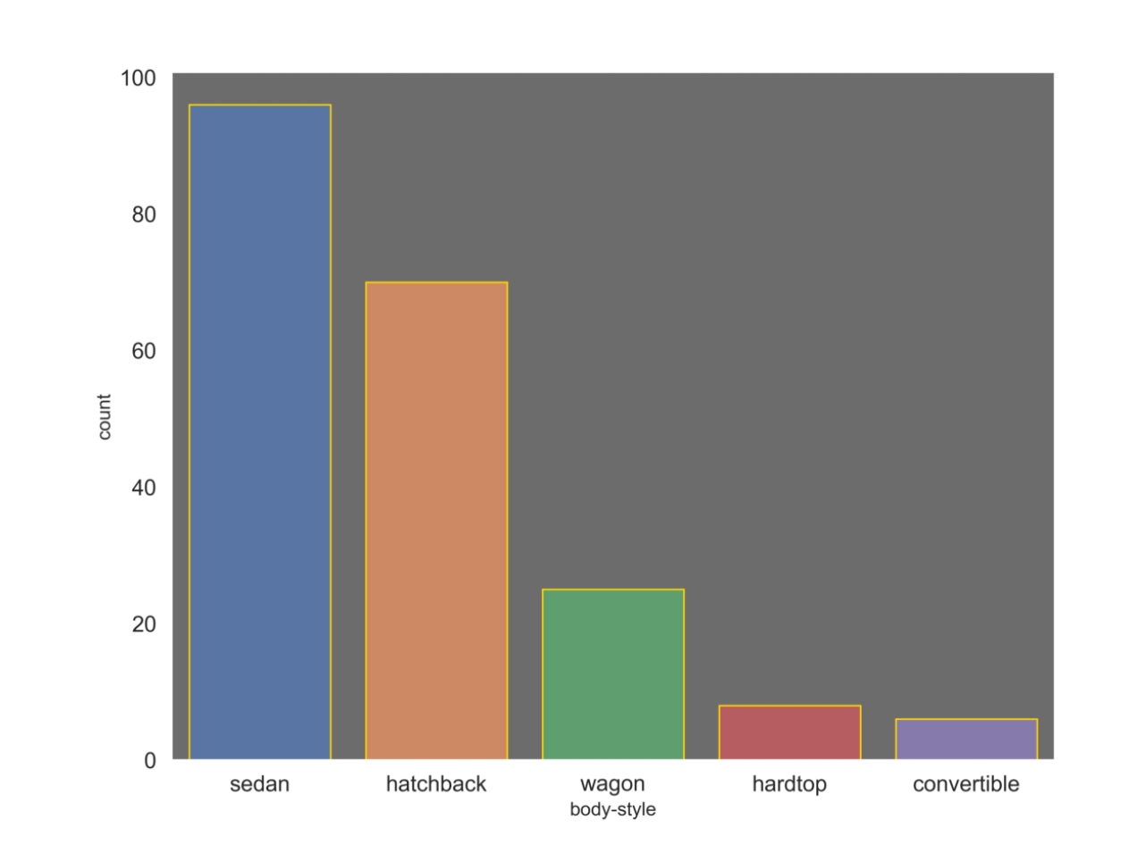
5.countplot
countplt用来绘制某个字段的数量分布信息.
1 | plt.figure(figsize=(10, 8)) |
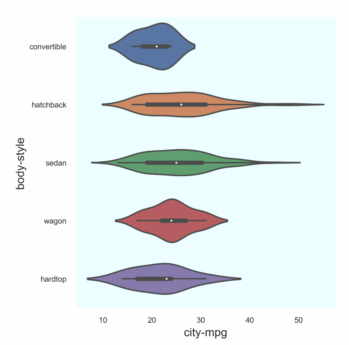
6. catplot
catplot本身是绘制类别分布情况,但是其可以绘制柱状图和violin,这个参数是kind。并且violin可以表示双变量。关于小提琴图和box图。
1 | sns.set(rc={ |
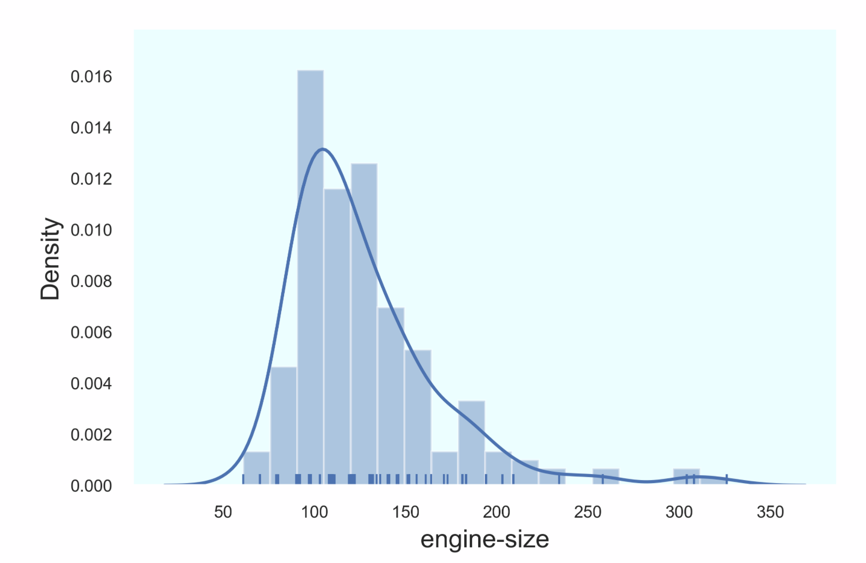
7.Dist plot
这部分主要是绘制histogram及核密度分布kernel density estimate(KDE)。
1 | sns.set(rc={ |
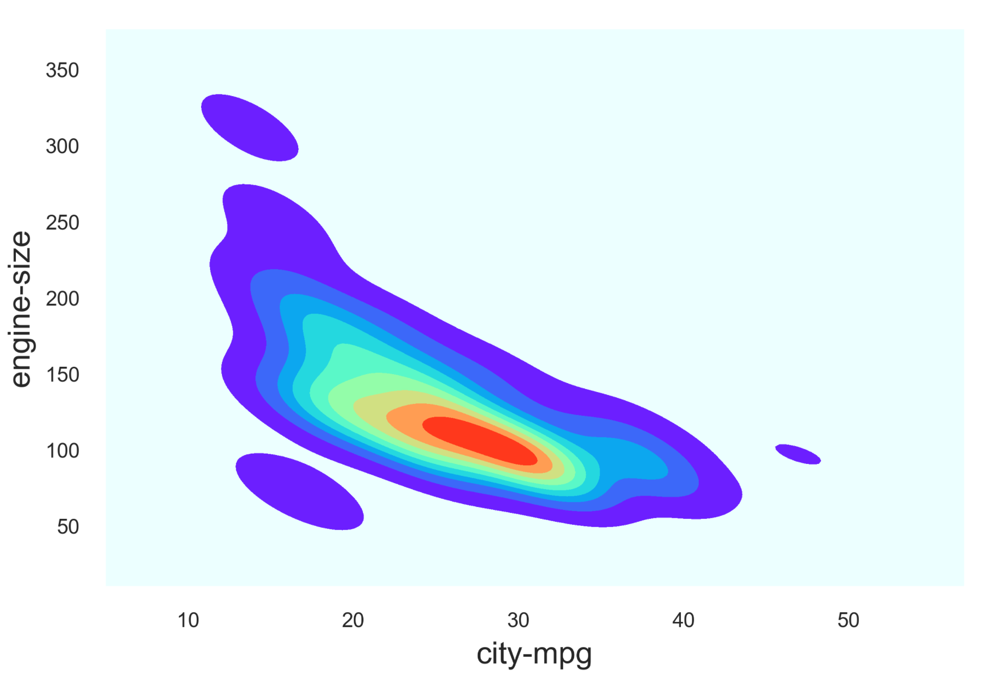
我们可以用kdeplot只绘制kde图, cmap 查询页.
1 | sns.kdeplot(auto['city-mpg'], auto['engine-size'], shade=True, cmap='rainbow', shade_lowest=False) |
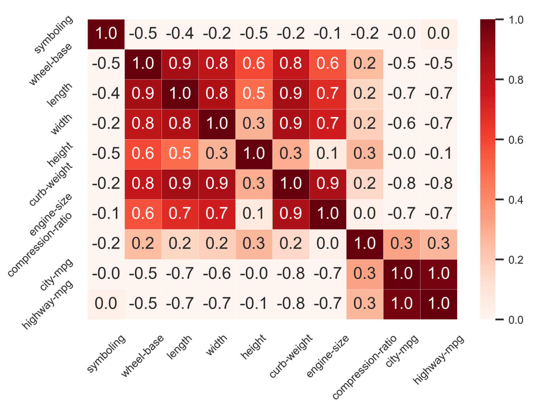
8. heatmap
一般用到热力图用来看相关性。参数主要有:
vmax:设置颜色带的最大值vmin:设置颜色带的最小值center:设置颜色带的分界线annot=True:小格子里填不填注释fmt:小格子里数据格式linewidths:小格子间间隔线宽度
1 | corr = auto.corr() |
Inference
[1] Seaborn Tutorial
 wechat
 alipay