Tabular Playground Series 比赛 去噪和quantile normalization 原文 ,利用自编码器去噪。
1. 导入包和数据 1 2 3 4 5 6 7 8 9 10 11 12 13 14 15 16 17 18 19 20 21 22 import random, math, sysimport numpy as npimport pandas as pdimport matplotlib.pyplot as plt%matplotlib inline from pathlib import Pathimport seaborn as snsimport tensorflow as tfimport tensorflow.keras.backend as Kfrom tensorflow import kerasfrom tensorflow.keras import layers, initializers, regularizers, activations, callbacksfrom tensorflow.keras.optimizers import Adamfrom tensorflow.keras.models import Modelimport tensorflow_addons as tfafrom sklearn.model_selection import KFold, StratifiedKFoldfrom sklearn.preprocessing import StandardScaler, scalefrom sklearn.metrics import mean_squared_errorfrom sklearn.model_selection import train_test_splitfrom sklearn.decomposition import PCAimport warningswarnings.simplefilter('ignore' )
使用版本信息:
1 2 3 4 5 print (tf.__version__)print (keras.__version__)=========================== 2.4 .1 2.4 .0
导入数据 :
1 2 3 4 5 6 7 8 9 10 11 12 13 data_dir = Path("/data" ) train = pd.read_csv(data_dir/'train.csv' ) test = pd.read_csv(data_dir/'test.csv' ) sample = pd.read_csv(data_dir/'sample_submission.csv' ) train.drop(['id' ], axis=1 , inplace=True ) test.drop(['id' ], axis=1 , inplace=True ) y = np.array(train['loss' ]) X = train.drop(['loss' ], axis=1 ) xall = pd.concat([X, test], axis=0 , copy=False ).reset_index(drop=True ) print (X.shape, y.shape, test.shape, xall.shape)================================================== (250000 , 100 ) (250000 ,) (150000 , 100 ) (400000 , 100 )
2. quantile normalize Quantile_normalization 解释,用它处理数据来得到相同分布。具体来说:
先分级,如例子中基因的数目为4就分为4个级别。
1 2 3 4 A 5 4 3 B 2 1 4 C 3 4 6 D 4 2 8
对应分配级别i-iv,记下对应的rank
1 2 3 4 A iv iii i B i i iiC ii iii iii D iii ii iv
对原始数据的按特征列排序。
1 2 3 4 A 5 4 3 becomes A 2 1 3 B 2 1 4 becomes B 3 2 4 C 3 4 6 becomes C 4 4 6 D 4 2 8 becomes D 5 4 8
对排序后的数据进行每行求均值
1 2 3 4 A (2 + 1 + 3 )/3 = 2.00 = rank i B (3 + 2 + 4 )/3 = 3.00 = rank iiC (4 + 4 + 6 )/3 = 4.67 = rank iii D (5 + 4 + 8 )/3 = 5.67 = rank iv
我们再按1中的对应的rank填入对应值, 到这儿就是quantile normalize算法过程。
1 2 3 4 A 5.67 4.67 2.00 B 2.00 2.00 3.00 C 3.00 4.67 4.67 D 4.67 3.00 5.67
实际过程中,步骤4中的第二列,有两个一样值4.67,这是要避免的,你要把每列都同分布嘛,就取和最靠近的哪个rank对应值的平均值。这就是具体quantile normalize过程,最后结果如下:
1 2 3 4 A 5.67 5.17 2.00 B 2.00 2.00 3.00 C 3.00 5.17 4.67 D 4.67 3.00 5.67
在该数据集中,我们直接先对原始数据进行类似最大最小化的75分位数25分位处理,来避免分位数归一化中的同数情况。#TODO1 2 3 4 5 6 7 8 9 10 11 12 13 14 15 16 17 xmedian = pd.DataFrame.median(xall, 0 ) x25quan = xall.quantile(0.25 , 0 ) x75quan = xall.quantile(0.75 , 0 ) xall = (xall- xmedian)/(x75quan-x25quan) def quantile_norm (df_input ): """分位数标准化""" sorted_df = pd.DataFrame(np.sort(df_input.values, axis=0 ), index=df_input.index, columns=df_input.columns) mean_df = sorted_df.mean(axis=1 ) mean_df.index = np.arange(1 , len (mean_df) + 1 ) quantile_df = df_input.rank(axis=0 , method='min' ).stack().astype('int' ).map (mean_df).unstack() return (quantile_df) qall = np.array(quantile_norm(xall)) qlabeled = qall[:len (train), :] qunlabled = qall[len (train):, :]
拿 quantile_norm(df_input)实验一下wiki例子:
1 2 3 4 5 6 7 8 xall = pd.DataFrame([[5 , 4 , 3 ], [2 , 1 , 4 ], [3 , 4 , 6 ], [4 , 2 , 8 ]]) qall = np.array(quantile_norm(xall)) print (qall)============================================= [[5.66666667 4.66666667 2. ] [2. 2. 3. ] [3. 4.66666667 4.66666667 ] [4.66666667 3. 5.66666667 ]]
3. creation bins 创建箱分位数据来进一步增加数据输入多样性。
1 2 3 4 5 6 7 ball = np.zeros((qall.shape[0 ], X.shape[1 ])) for i in range (X.shape[1 ]): ball[:, i] = pd.qcut(qall[:, i], X.shape[1 ], labels=False , duplicates='drop' ) blabled = ball[:X.shape[0 ], :] bunlabled = ball[X.shape[0 ]:, :]
例如拿wiki例子中数据,就是上面 [5.66666667 4.66666667 2. ]这个矩阵, 来处理下有:
1 2 3 4 5 6 7 8 9 ball = np.zeros((qall.shape[0 ], qall.shape[1 ])) for i in range (qall.shape[1 ]): ball[:, i] = pd.qcut(qall[:, i], qall.shape[1 ], labels=False , duplicates='drop' ) print (ball)=================================== [[2. 1. 0. ] [0. 0. 0. ] [0. 1. 1. ] [1. 0. 2. ]]
4. denoise Autoencoder 1 2 3 4 5 6 7 8 9 10 11 12 13 14 15 16 17 18 19 20 21 22 23 24 25 26 27 28 29 30 31 32 33 34 35 36 37 38 39 40 41 42 43 44 45 46 47 48 49 50 noise = np.random.normal(0 , .1 , (qall.shape[0 ], qall.shape[1 ])) qall = np.array(qall) xnoisy = qall + noise limit = np.int (0.8 * qall.shape[0 ]) xtrain = xnoisy[0 :limit, :] ytrain = qall[0 :limit, ] xval = xnoisy[limit:qall.shape[0 ], :] yval = qall[limit:qall.shape[0 ], :] print (xtrain.shape, ytrain.shape, xval.shape, yval.shape)====================================================== (320000 , 100 ) (320000 , 100 ) (80000 , 100 ) (80000 , 100 ) es = tf.keras.callbacks.EarlyStopping( monitor='val_loss' , min_delta=1e-9 , patience=20 , verbose=0 , mode='min' , baseline=None , restore_best_weights=True ) plateau = tf.keras.callbacks.ReduceLROnPlateau( monitor='val_loss' , factor=0.8 , patience=4 , verbose=0. , mode='min' ) def custom_loss (y_true, y_pred ): loss = K.mean(K.square(y_pred - y_true)) return loss def autoencoded (): ae_input = layers.Input(shape=(qall.shape[1 ])) ae_encoded = layers.Dense(units=qall.shape[1 ], activation='elu' )(ae_input) ae_encoded = layers.Dense(units=qall.shape[1 ]*3 , activation='elu' )(ae_encoded) ae_decoded = layers.Dense(units=qall.shape[1 ], activation='elu' )(ae_encoded) return Model(ae_input, ae_decoded), Model(ae_input, ae_encoded) autoencoder, encoder = autoencoded() autoencoder.compile (loss=custom_loss, optimizer=keras.optimizers.Adam(lr=5e-3 ))
自编码器的总结:
1 2 3 4 5 6 7 8 9 10 11 12 13 14 15 16 17 autoencoder.summary() =========================== Model: "model" _________________________________________________________________ Layer (type ) Output Shape Param ================================================================= input_1 (InputLayer) [(None , 100 )] 0 _________________________________________________________________ dense (Dense) (None , 100 ) 10100 _________________________________________________________________ dense_1 (Dense) (None , 300 ) 30300 _________________________________________________________________ dense_2 (Dense) (None , 100 ) 30100 ================================================================= Total params: 70 ,500 Trainable params: 70 ,500 Non-trainable params: 0
训练自编码器1 2 3 4 5 6 7 8 9 10 history = autoencoder.fit(xtrain, ytrain, epochs=200 , batch_size=512 , verbose=0 , validation_data=(xval, yval), callbacks=[es, plateau]) eall = encoder.predict(qall) print ("max encoded value = " , np.max (eall))print (eall.shape)
5. 根据方差阈值特征编码选择特征 1 2 3 4 5 6 7 8 9 10 11 12 13 14 15 16 17 18 evar = np.var(eall, axis=0 , ddof=1 ) evar1 = evar > 0.8 a = np.where(evar1 == False , evar1, 1 ) nb_col = a.sum () eall_1 = pd.DataFrame() for i in range (qall.shape[1 ] * 3 ): if evar1[i] == True : colname = f'col_{i} ' eall_1[colname] = eall[:, i] eall_1 = np.array(eall_1) elabeled = eall_1[:len (train), :] eunlabeled = eall_1[len (train):, :] elabeled.shape, eunlabeled.shape ================================= ((250000 , 100 ), (150000 , 100 ))
6. 对编码特征进行PCA降维再标准化 1 2 3 4 pca = PCA(n_components=15 ) pall = pca.fit_transform(eall) sc_pca = StandardScaler() pall = sc_pca.fit_transform(pall)
7.合并PCA降维后特征和编码特征(方差阈值之后) 1 2 3 4 plabled = pall[:len (train), :] punlabled = pall[len (train):, :] elabeled = np.hstack((elabeled, plabled)) eunlabeled = np.hstack((eunlabeled, punlabled))
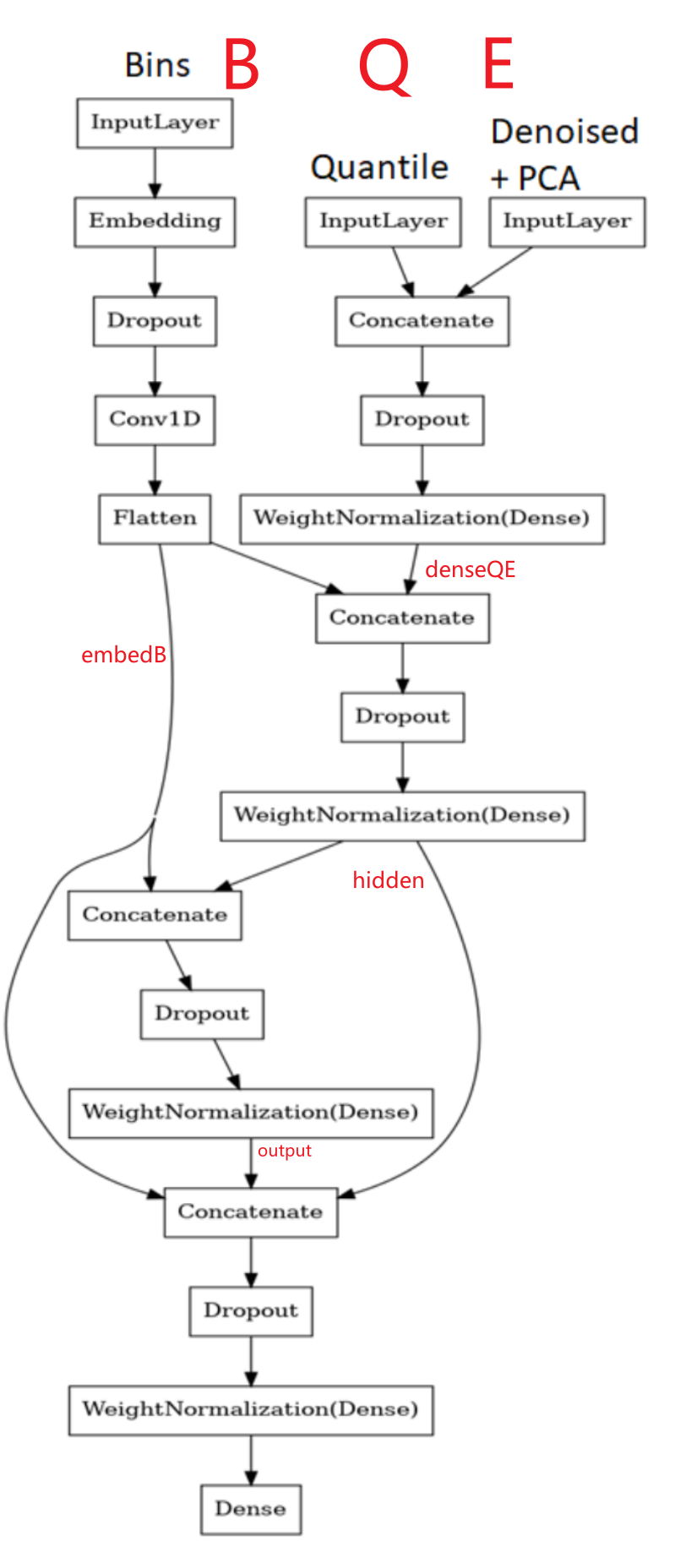
8. 构建残差模型来解决任务 这块很有意思搭建多残差网络,根据图来理解
1 2 3 4 5 6 7 8 9 10 11 12 13 14 15 16 17 18 19 20 21 22 23 24 25 26 27 28 29 30 31 32 33 34 35 36 37 38 39 40 41 42 43 44 45 46 47 48 49 50 51 52 53 54 55 def get_res_model (): inputQ = layers.Input(shape=(qall.shape[1 ])) inputE = layers.Input(shape=(elabeled.shape[1 ])) inputB = layers.Input(shape=(blabled.shape[1 ])) denseQE = layers.Dropout(0.3 )(layers.Concatenate()([inputQ, inputE])) denseQE = tfa.layers.WeightNormalization(layers.Dense( units=300 , activation='elu' , kernel_initializer='lecun_normal' ))(denseQE) embedB = layers.Embedding(input_dim=blabled.shape[1 ] + 1 , output_dim=6 , embeddings_regularizer='l2' , embeddings_initializer='lecun_uniform' )(inputB) embedB = layers.Dropout(0.3 )(embedB) embedB = layers.Conv1D(6 , 1 , activation='relu' )(embedB) embedB = layers.Flatten()(embedB) hidden = layers.Dropout(0.3 )(layers.Concatenate()([denseQE, embedB])) hidden = tfa.layers.WeightNormalization(layers.Dense( units=64 , activation='elu' , kernel_initializer='lecun_normal' ))(hidden) output = layers.Dropout(0.3 )(layers.Concatenate()([embedB, hidden])) output = tfa.layers.WeightNormalization( layers.Dense(units=32 , activation='relu' , kernel_initializer='lecun_normal' ) )(output) output = layers.Dropout(0.4 )(layers.Concatenate()([embedB, hidden, output])) output = tfa.layers.WeightNormalization(layers.Dense( units=32 , activation='selu' , kernel_initializer='lecun_normal' ))(output) output = layers.Dense(units=1 , activation='selu' ,\ kernel_initializer='lecun_normal' )(output) model = Model([inputQ, inputE, inputB], output) model.compile (loss='mse' , metrics=[tf.keras.metrics.RootMeanSquaredError()], optimizer=keras.optimizers.Adam(lr=0.005 )) return model
9. 训练模型 1 2 3 4 5 6 7 8 9 10 11 12 13 14 15 16 17 18 19 20 21 22 23 24 25 26 27 28 29 30 31 32 33 34 35 36 37 38 39 40 41 42 43 44 45 46 47 48 49 50 51 52 53 N_FOLDS = 10 SEED = 1 EPOCH = 100 N_ROUND = 5 oof = np.zeros((y.shape[0 ], 1 )) pred = np.zeros((test.shape[0 ], 1 )) for i in range (N_ROUND): oof_round = np.zeros((y.shape[0 ], 1 )) skf = StratifiedKFold(n_splits=N_FOLDS, shuffle=True , random_state=SEED*i) for fold, (tr_idx, ts_idx) in enumerate (skf.split(X, y)): print (f"\n ---------Training Round {i+1 } Fold {fold+1 } ----\n" ) qtrain = qlabeled[tr_idx] qval = qlabeled[ts_idx] btrain = blabled[tr_idx] bval= blabled[ts_idx] etrain = elabeled[tr_idx] eval = elabeled[ts_idx] ytrain = y[tr_idx] yval = y[ts_idx] K.clear_session() nn_model = get_res_model() nn_model.fit([qtrain, etrain, btrain], ytrain, batch_size=2048 , epochs=EPOCH, validation_data=([qval, eval , bval], yval), callbacks=[es, plateau], verbose=1 ) nn_model.save(data_dir/f'model{i} .ckpt' ) pred_round = nn_model.predict([qval, eval , bval]) oof[ts_idx] += pred_round / N_ROUND oof_round[ts_idx] += pred_round pred += nn_model.predict([qunlabled, eunlabeled, bunlabled]) / (N_FOLDS * N_ROUND) score_round = math.sqrt(mean_squared_error(y, oof_round)) print (f"第{i+1 } 轮分数{score_round} =====\n" ) score_round = math.sqrt(mean_squared_error(y, oof)) print (f"最终分数{score_round} =====\n" )
10. 预测 1 2 3 4 5 6 sample_submission = pd.read_csv(data_dir/'sample_submission.csv' ) sample_submission['pred' ] = pred pd.DataFrame(oof).to_csv('oof.csv' , index=False ) sample_submission.to_csv('sb1.csv' , index=False ) display(pd.read_csv('sb1.csv' ))
 wechat
 alipay