RNN, LSTM , GRU 结构解释和其在Pytorch中的使用
1. RNN 结构和内部计算
RNN结构示意图(这里没画bias, 但公式里写了,借的李宏毅教授PPT图)
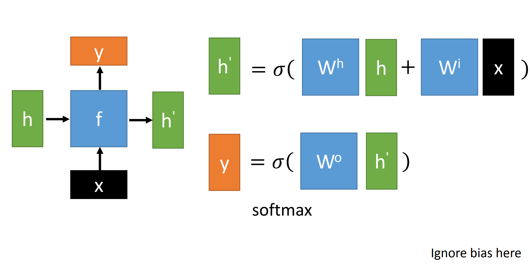
$x$为当前状态下数据的输入, $h$表示接收到的上一个节点的输入。
$y$为当前节点状态下的输出,而 $h^{\prime} $为传递到下一个节点的输出。
真实计算公式为:
通过上图的公式可以看到,输出$\boldsymbol{h}^{\prime}$与 $\boldsymbol{x}$ 和 $\boldsymbol{h}$的值都相关。
而 $\boldsymbol{y}$ 则常常使用 $\boldsymbol{h}^{\prime}$投入到一个线性层(主要是进行维度映射)然后使用softmax进行分类得到需要的数据。
对这里的$\boldsymbol{y}$如何通过 $\boldsymbol{h}^{\prime}$ 计算得到往往看具体模型的使用方式。
简单使用rnn实例如下:
1
2
3
4
5
6
7
8
9
10
11
12
13
14
|
rnn = nn.RNN(input_size=20,hidden_size=50,num_layers=2)
input_data = Variable(torch.randn(100,32,20))
h_0 = Variable(torch.randn(2,32,50))
output,h_t = rnn(input_data,h_0)
print(output.size())
print(h_t.size())
print(rnn.weight_ih_l0.size())
++++++++++++++++++++++++++++++++++++++++++++++
torch.Size([100, 32, 50])
torch.Size([2, 32, 50])
torch.Size([50, 20])
|
通过序列形式的输入,我们能够得到如下形式的RNN。
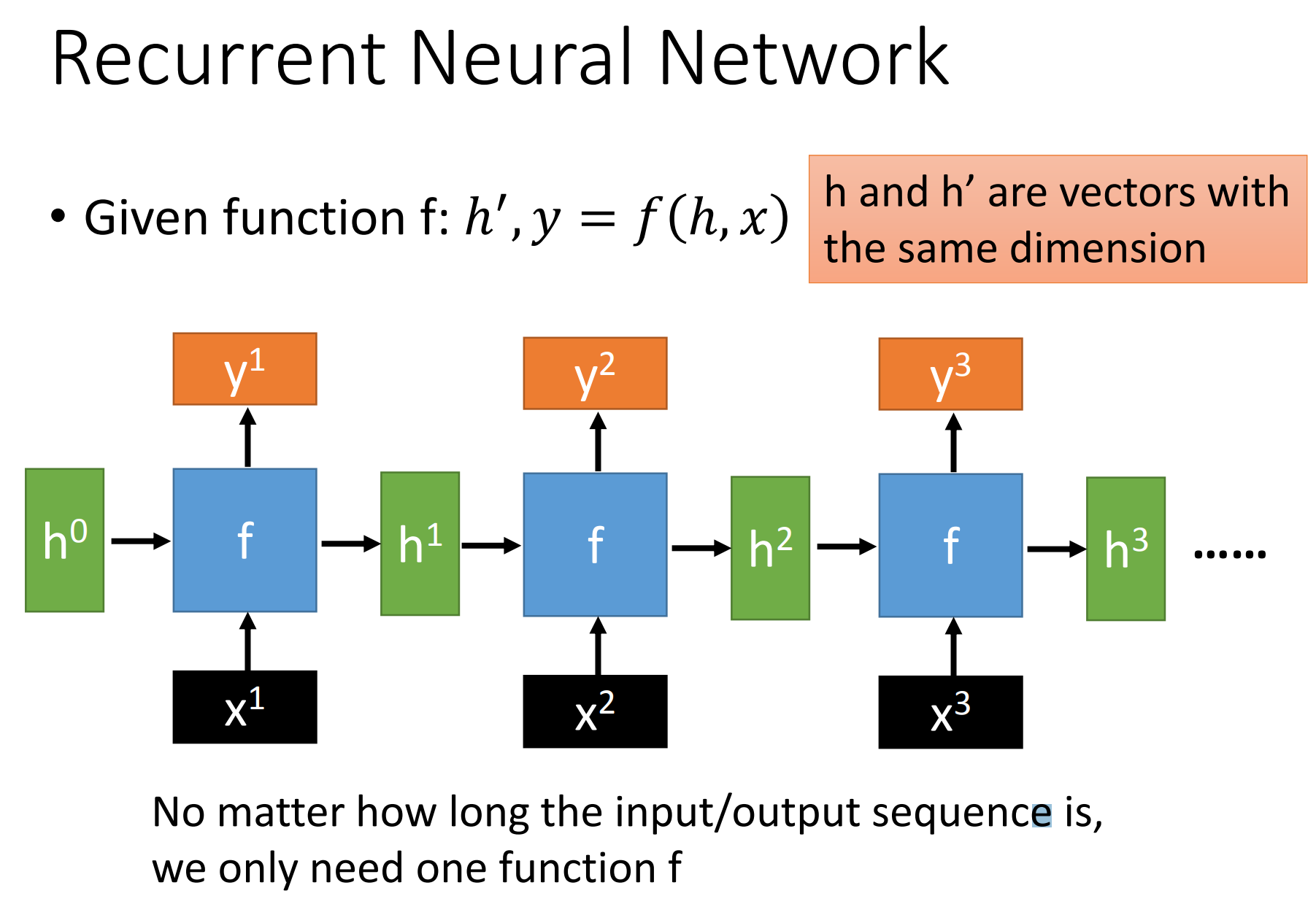
序列模型中RNN的搭建:
使用 nn.RNN(input_size, hidden_size, num_layers)中参数解释
- input_size – The number of expected features in the input x
- hidden_size – The number of features in the hidden state h
- num_layers – Number of recurrent layers.
- bidirectional –
If True, becomes a bidirectional RNN. Default: False
输出是$y_t, h_t$
1
2
3
4
5
6
7
8
9
10
11
12
13
14
15
16
17
18
19
20
21
22
23
24
25
26
27
28
29
30
31
32
33
34
35
36
37
38
| class RNN(nn.Module):
def __init__(self, input_size, hidden_size, output_size, num_layers=1):
super(RNN, self).__init__()
"""
分别代表输入最后一维尺寸
隐藏层最后一维尺寸
输出层最后一维尺寸
层数
"""
self.input_size = input_size
self.hidden_size = hidden_size
self.output_size = output_size
self.num_layers = num_layers
self.rnn = nn.RNN(input_size, hidden_size, num_layers)
self.linear = nn.Linear(hidden_size, output_size)
self.softmax = nn.LogSoftmax(dim=-1)
def forward(self, input1, hidden):
"""
:param input: 输入, 1xn_letters
:param hidden: 隐藏层张量, self.layers x 1 x self.hidden_size
:return:
"""
input1 = input1.unsqueeze(0)
rr, hn = self.rnn(input1, hidden)
return self.softmax(self.linear(rr)), hn
def initHidden(self):
return torch.zeros(self.num_layers, 1, self.hidden_size)
|
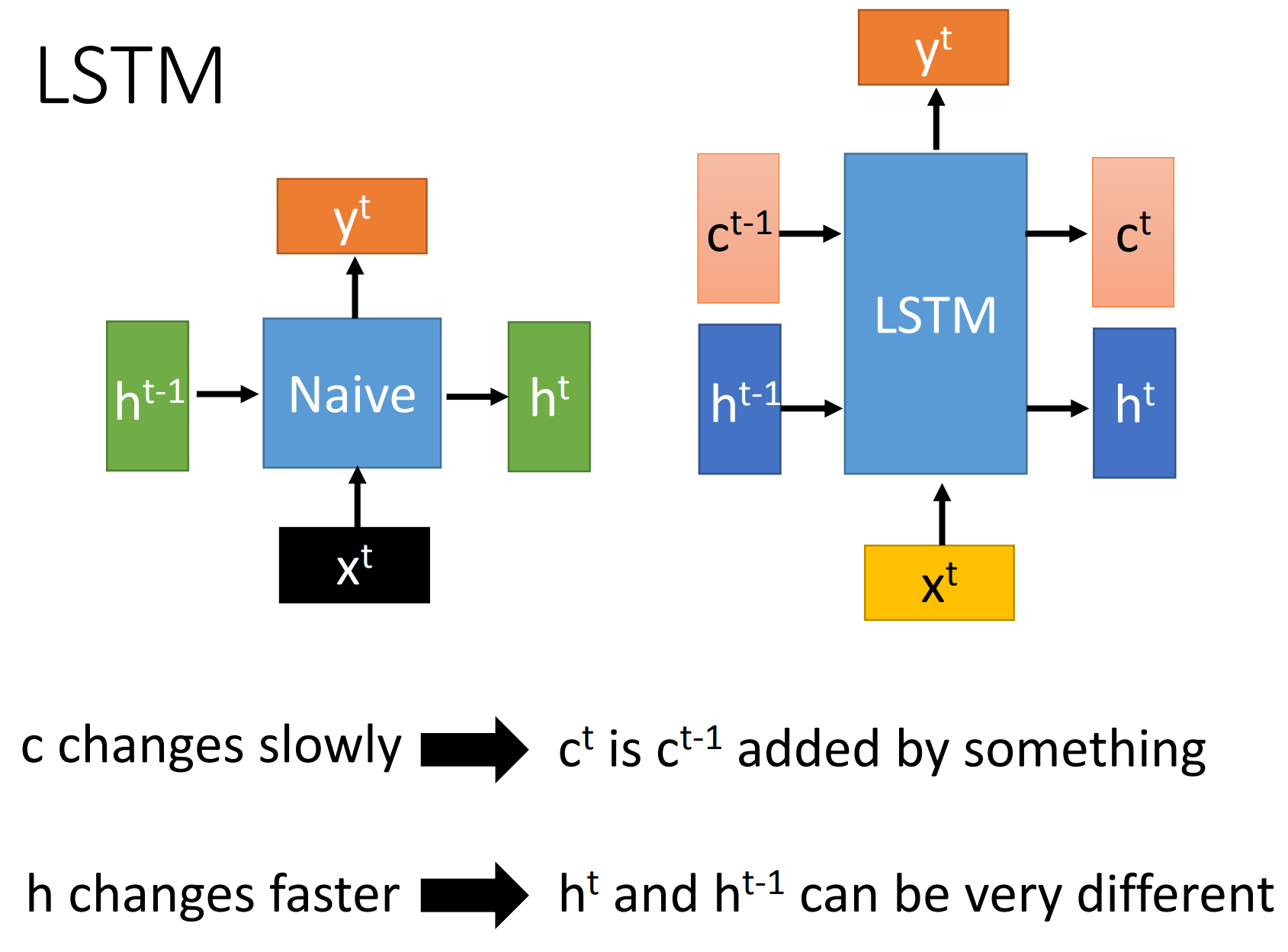
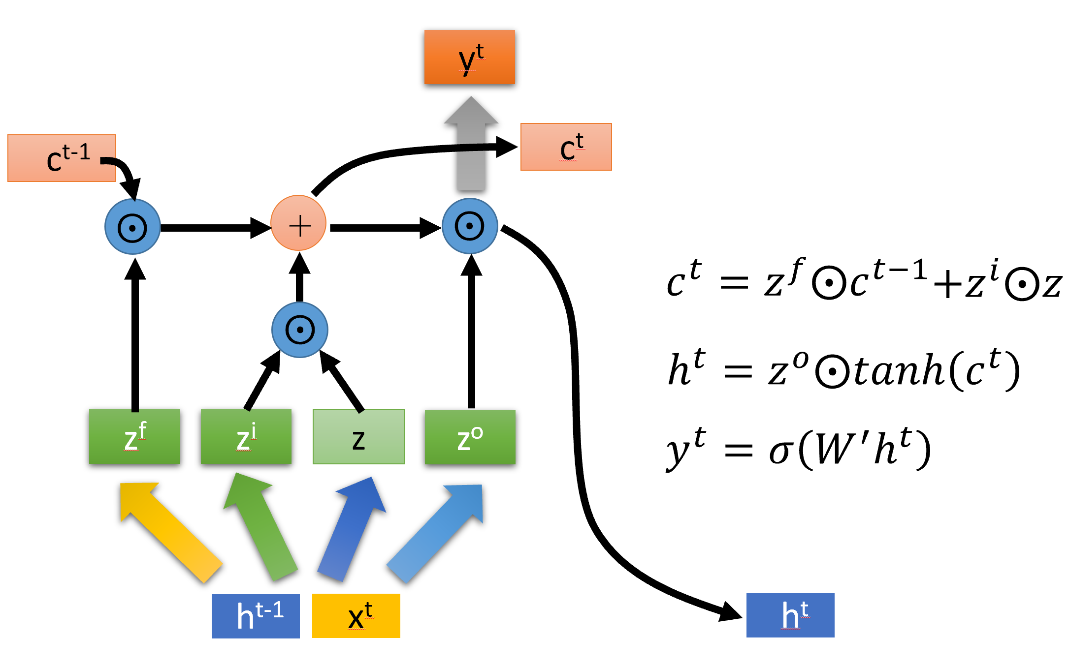
2. LSTM
LSTM是long short-term memory,与RNN区别是
- LSTM两个传递状态:$c^t $ cell state, $h^t$ hidden state
- RNN一个传递状态: $h^t$
注: RNN中$h^t$等价于 LSTM中 $c^t$
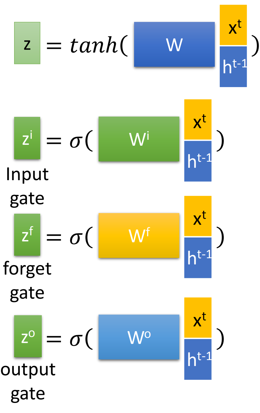
而对于input gate, forget gate, output gate中是$[x^t, h^{t-1}]$向量拼接后乘以相应权重矩阵再过sigmoid函数转换为0到1的数值,作为门控状态。
需要注意的是z是tanh函数,转换为-1到1,因为是输入数据不是门控状态。
因此有下面4个公式:(忽略bias)
注:[]表示两个向量拼接,而 $\boldsymbol{W}$四个权重矩阵都是训练学习得到的。
然后根据上面四个信号$ \boldsymbol{z}, \boldsymbol{z}^f, \boldsymbol{z}^i, \boldsymbol{z}^o $, 由下列公式得到输出, cell state和隐藏状态。
- cell state :等于 上一个cell state 与遗忘门信号 $\boldsymbol{z}^f $ Hadamard product,和 输入门信号 $ \boldsymbol{z}^i $与输入信号$\boldsymbol{z}$ 的Hadamard product之和
- hidden state: 等于输出门信号 $\boldsymbol{z}^o $ 与 过tanh后的 cell state 的Hadamard product
- 输出: 等于上一个时间步后权重矩阵$\boldsymbol{W}$ 与 隐藏状态过sigmoid
Pytorch中LSTM实例使用:
1
2
3
4
5
6
7
8
9
10
11
12
13
14
15
16
17
18
19
20
21
22
23
24
25
26
27
28
29
30
| lstm = nn.LSTM(input_size=20,hidden_size=50,num_layers=2)
input_data = Variable(torch.randn(100,32,20))
h_0 = Variable(torch.randn(2,32,50))
c_0 = Variable(torch.randn(2,32,50))
output,(h_t,c_t) = lstm(input_data,(h_0,c_0))
print(output.size())
print(h_t.size())
print(c_t.size())
print(lstm.weight_ih_l0)
print(lstm.weight_ih_l0.size())
++++++++++++++++++++++++++++++++++++++++++++++++++++++++++++++++++++++++++++++++++++++++++
torch.Size([100, 32, 50])
torch.Size([2, 32, 50])
torch.Size([2, 32, 50])
Parameter containing:
tensor([[ 0.1123, -0.0734, -0.0408, ..., -0.0715, 0.0920, 0.0409],
[-0.1310, -0.0566, -0.0761, ..., -0.0909, 0.0081, -0.0258],
[ 0.0264, 0.0297, 0.0800, ..., 0.0869, -0.0008, -0.0621],
...,
[-0.0116, 0.0778, -0.1181, ..., 0.1066, 0.0610, 0.0846],
[ 0.0216, -0.0159, 0.1354, ..., 0.0726, -0.0238, -0.1158],
[-0.1081, -0.0760, -0.0722, ..., 0.0506, 0.0550, 0.1033]],
requires_grad=True)
torch.Size([200, 20])
|
在seq2seq任务中,使用:
1
2
3
4
5
6
7
8
9
10
11
12
13
14
15
16
17
18
19
20
21
22
23
24
25
26
27
28
29
30
31
32
33
34
35
36
37
38
39
40
41
| class LSTM(nn.Module):
def __init__(self, input_size, hidden_size, output_size, num_layers=1):
super(LSTM, self).__init__()
"""
分别代表输入最后一维尺寸
隐藏层最后一维尺寸
输出层最后一维尺寸
层数
"""
self.input_size = input_size
self.hidden_size = hidden_size
self.output_size = output_size
self.num_layers = num_layers
self.lstm = nn.LSTM(input_size, hidden_size, num_layers)
self.linear = nn.Linear(hidden_size, output_size)
self.softmax = nn.LogSoftmax(dim=-1)
def forward(self, input1, hidden, c):
"""
LSTM输入有3个
:param input1: 输入, 1xn_letters
:param hidden: 隐藏层张量, self.layers x 1 x self.hidden_size
:param c 张量, self.layers x 1 x self.hidden_size
:return:
"""
input1 = input1.unsqueeze(0)
rr, (hn, cn) = self.lstm(input1, (hidden, c))
return self.softmax(self.linear(rr)), hn, cn
def initHidden(self):
c = hidden = torch.zeros(self.num_layers, 1, self.hidden_size)
return hidden, c
|
3. GRU
GRU(Gate Recurrent Unit)结构示意图如下:
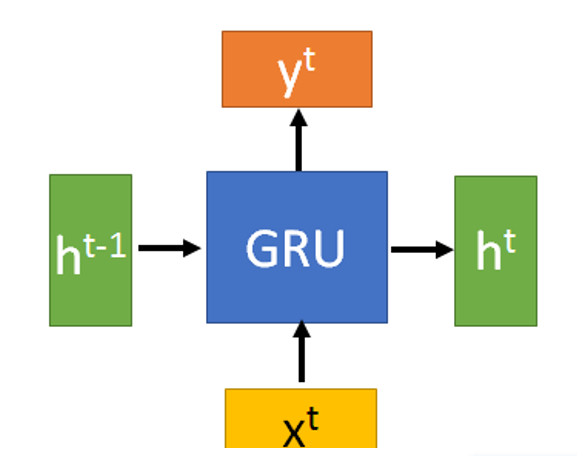
最重要的是,两个门控reset gate 和 update gate:
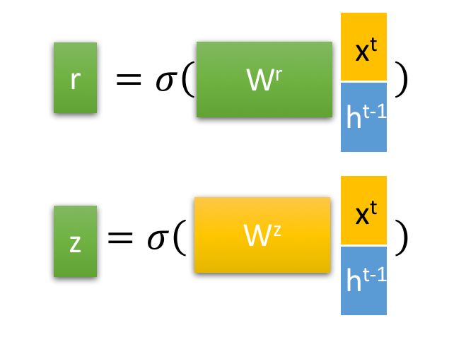
然后得到重置的隐藏层状态${\boldsymbol{h}^{t-1}}^\prime= \boldsymbol{h}^{t-1} \odot\boldsymbol{r}^{t} $. 将这个隐藏状态与$\boldsymbol{x}^t$ 拼接再过tanh将重置的隐藏状态缩放为-1~1.得到${\boldsymbol{h}^{t}}^\prime$
即
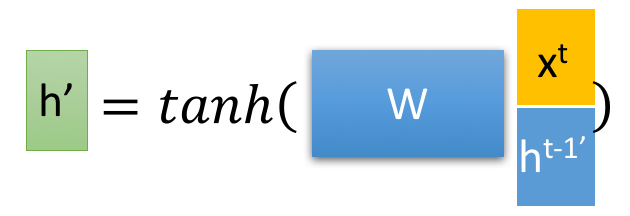
这里${\boldsymbol{h}^{t}}^\prime$ 主要包含了当前输入$ {\boldsymbol{x}^{t}} $数据, 还有有选择地添加上一个时间隐藏状态,这里主要是重置门信号作用(你可以理解为乘以一个0~1的数来控制添加隐藏状态的多少)。
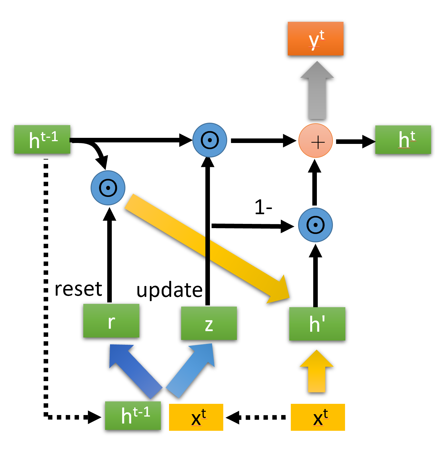
最后一步是$\boldsymbol{h}^{t}$,也是输出。计算公式为:
实际上,GRU是用一个update gate来替换LSTM的input gate 和 forget gate.
在 LSTM 中这两个门分别是
- 控制输入多少(输入是上一个时间状态和当前输入总的信息量)
- 控制遗忘信息量的多少
而update gate就是上面的$\boldsymbol{z}^t$ ,是一个0~1的控制信号。那么:
- $\boldsymbol{z}^t $理解等价于input gate 控制信号, $\boldsymbol{z}^t \odot {\boldsymbol{h}^{t}}^\prime$ 就等效于经过input gate后的信息
- $(1-\boldsymbol{z}^t )$ 等价于 forget gate 控制信号, $(1-\boldsymbol{z}^t ) \odot \boldsymbol{h}^{t-1}$ 等效于 经过 forget gate后的信息
1
2
3
4
5
6
7
8
9
10
11
12
13
14
15
16
17
18
19
20
21
22
23
24
25
26
| gru = nn.GRU(input_size=20,hidden_size=50,num_layers=2)
input_data = Variable(torch.randn(100,32,20))
h_0 = Variable(torch.randn(2,32,50))
output,(h_n,c_n) = gru(input_data)
print(output.size())
print(h_n.size())
print(gru.weight_ih_l0)
print(gru.weight_ih_l0.size())
+++++++++++++++++++++++++++++++++++++++++++++++++++++++++++++++++++++++++
torch.Size([100, 32, 50])
torch.Size([32, 50])
Parameter containing:
tensor([[ 0.0465, 0.0917, 0.1357, ..., -0.1283, 0.1264, -0.0320],
[ 0.1384, 0.1072, 0.0073, ..., -0.0772, -0.1295, 0.0233],
[-0.0627, -0.1012, -0.0415, ..., 0.1311, 0.1374, -0.0566],
...,
[-0.0131, 0.0995, 0.0054, ..., -0.0350, -0.1220, 0.1143],
[-0.0836, 0.1239, 0.0860, ..., 0.0837, 0.0172, -0.0170],
[ 0.0637, 0.0501, 0.0091, ..., -0.1201, 0.0788, 0.0468]],
requires_grad=True)
torch.Size([150, 20])
|
seq2seq中使用:
1
2
3
4
5
6
7
8
9
10
11
12
13
14
15
16
17
18
19
20
| class GRU(nn.Module):
def __init__(self, input_size, hidden_size, output_size, num_layers=1):
super(GRU, self).__init__()
self.input_size = input_size
self.hidden_size = hidden_size
self.num_layers = num_layers
self.output_size = output_size
self.gru = nn.GRU(input_size, hidden_size, num_layers)
self.linear = nn.Linear(hidden_size, output_size)
self.softmax = nn.LogSoftmax(dim=-1)
def forward(self, input, hidden):
input = input.unsqueeze(0)
rr, hn = self.gru(input, hidden)
return self.softmax(self.linear(rr)), hn
def initHidden(self):
return torch.zeros(self.num_layers, 1, self.hidden_size)
|
Inference
[1] Seq-to-seq Learning.pdf )
[2] 人人都能看懂的LSTM
[3] NLP: text classification 图示漂亮
 wechat
 alipay