机器学习-白板推导 4.1 线性分类 1. 从线性回归到线性分类 线性回归的特性及将线性回归转为线性分类的办法
线性回归模型可以写作。其线性体现在三个方面:
属性线性:关于 是线性的
全局线性:指是一个线性组合,然后输出得到
系数线性:指 关于也是线性的
如果将某一种线性改为非线性就可以得到一种非线性模型。对应有:
将属性改为非线性 :可以用特征转换(多项式回归),如
将全局线性改为非线性 :加入激活函数,让输出变成非线性,比如logistic 分类,就变成了线性分类
将系数线性改为非线性 :系数会改变,比如神经网络,通过反向传播改变权重。
而线性回归还有全局性 和数据未加工 的特性:
全局性 :指线性回归是在整个特征空间上学习的,并没有将特征空间进行划分,然后在每个特征上学习。数据未加工 :线性回归直接在给定数据上进行学习而没有对数据进行处理,如PCA,流形等。
将全局性打破 ,即不根据所有点的情况回归,而是将数据分为一个个小的空间,对每个子空间进行回归,如决策树模型。
总结 :
线性分类分类 :
2. 感知机
概述
假设有一可被线性分类的样本集,其中.那么感知机算法可以使用SGD来在特征空间中找到一个超平面可以将其分为两类,其中,是这个超平面的法向量。
感知机算法是错误驱动的算法,可以理解为不断调整这个超平面来使得误分类错误点越少。
具体算法
对于所有的样本数据:
可直接改写为代表正确分类,反之就是错误分类。
而特征空间中任意一点到超平面的距离为 :
所有误分类点到超平面总距离为:
不考虑,就可以得到感知机损失函数:
学习算法
对损失函数求梯度得:
实际训练步骤如下( ):[李航——统计学习方法P39]
选取初值
在训练集中选取数据
如果, 则更新参数:
转至2,直到训练集中没有误分类点
3. 线性判别分析
算法思想
假设数据集为, 其中 ,,记 为 类,为类。那么,为,为, 且。
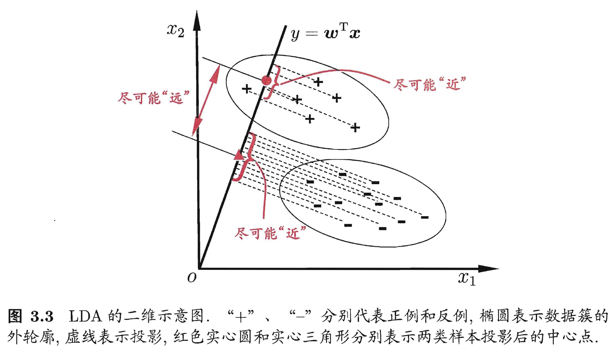
LDA (Linear Discriminant Analysis) 的想法是: 设法将数据样本投影到一条直线上,使得同类别样本的投影点尽可能接近、异类样本投影点尽可能远。总结来说就是, 类内小、类间大,具体是指类内方差之和小,类间的均值之差大。具体图示如下:(出自: 周志华——《机器学习》”西瓜书“ P60)
算法推导
若将数据投影到直线上,则样本点投影到该直线后值为。样本均值和方差按以下公式计算:
那么对于第一类分类点和第二类分类点可以表述为:
那么类间的距离我们可以定义为:$(\bar{z_1}-\bar{z_2})^2$,
根据目标函数要使得分子越小越好,分母越大越好。即类间距离越大越好,类内的距离越小越好。
分子 化简:
分母化简 :
同理可得,
所以, 分母化简为。代入目标函数得:
定义类间散度矩阵为(within-class scatter matrix):
类内散度矩阵为(between-class scatter matrix):
于是,目标函数改写为:
为了方便求导,我们令 。
显然,$w$的维度是$p\times 1$,$w^T$的维度是$1 \times p$,$S_w$的维度是$p\times p$,所以,$w^TS_ww$是一个实数,同理 可得,$w^TS_ww$是一个实数所以,
我们只要方向,大小由于超平面可以放缩,可以不关注。可以忽略一些实数,
而代入有:
因为也是个实数,可以忽略。所以最后正比于:
那么,我们最后求得方向为。如果对角矩阵是各项同性,那么其正比于单位矩阵,,则有。
实际分类中很少用LDA了,但是其在早期是非常有代表性的算法,可以参考其思想。
3. 逻辑回归 逻辑回归的想法是,我们将线性回归得到的值经过一个函数映射后能不能得到一个在的值,这样可以将其看作一个概率值。而sigmoid恰好有这个性质,其定义为:
如图所示:
算法推导 :
假设数据集为:。
记:
简化后记为:
只要对于所有样本的概率最大就是最优参数,用MLE求解最优:
最后的 也可以根据交叉熵公式写出,不过要加个负号。
现在只要求解最大值。
其中,表达式如上,并且对sigmoid求导有,因此有:
令其为0时,可求出。但是由于概率是非线性的,该式无法实际求解,实际上使用SGD来求最大值。当最优解为时,
其中,
代码实现:引用自[zhulei227] 02线性模型 逻辑回归.ipynb
1
2
3
4
5
6
7
8
9
10
11
12
13
14
15
16
17
18
19
20
21
22
23
24
25
26
27
28
29
30
31
32
33
34
35
36
37
38
39
40
41
42
43
44
45
46
47
48
49
50
51
52
53
54
55
56
57
58
59
60
61
62
63
64
65
66
67
68
69
70
71
72
73
74
75
76
77
78
79
80
81
82
83
84
85
86
87
88
89
90
91
92
93
94
95
96
97
98
99
100
101
102
103
104
105
106
107
108
109
110
111
112
113
114
115
116
117
118
119
120
121
122
123
124
125
126
127
128
129
130
131
132
133
134
135
136
137
138
139
140
141
142
143
144
145
146
147
148
149
150
151
152
class LogisticRegression (object ): def __init__ (self, fit_intercept=True , solver='sgd' , if_standard=True , l1_ratio=None , l2_ratio=None , epochs=10 , eta=None , batch_size=16 ): self.w = None self.fit_intercept = fit_intercept self.solver = solver self.if_standard = if_standard if if_standard: self.feature_mean = None self.feature_std = None self.epochs = epochs self.eta = eta self.batch_size = batch_size self.l1_ratio = l1_ratio self.l2_ratio = l2_ratio self.sign_func = np.vectorize(utils.sign) self.losses = [] def init_params (self, n_features ): """ 初始化参数 w """ self.w = np.random.random(size=(n_features, 1 )) def _fit_closed_form_solution (self, x, y ): """ 直接求闭式解 """ self._fit_sgd(x, y) def _fit_sgd (self, x, y ): """ 随机梯度下降求解 """ x_y = np.c_[x, y] count = 0 for _ in range (self.epochs): np.random.shuffle(x_y) for index in range (x_y.shape[0 ] // self.batch_size): count += 1 batch_x_y = x_y[self.batch_size * index:self.batch_size * (index + 1 )] batch_x = batch_x_y[:, :-1 ] batch_y = batch_x_y[:, -1 :] dw = -1 * (batch_y - utils.sigmoid(batch_x.dot(self.w))).T.dot(batch_x) / self.batch_size dw = dw.T dw_reg = np.zeros(shape=(x.shape[1 ] - 1 , 1 )) if self.l1_ratio is not None : dw_reg += self.l1_ratio * self.sign_func(self.w[:-1 ]) / self.batch_size if self.l2_ratio is not None : dw_reg += 2 * self.l2_ratio * self.w[:-1 ] / self.batch_size dw_reg = np.concatenate([dw_reg, np.asarray([[0 ]])], axis=0 ) dw += dw_reg self.w = self.w - self.eta * dw cost = -1 * np.sum ( np.multiply(y, np.log(utils.sigmoid(x.dot(self.w)))) + np.multiply(1 - y, np.log( 1 - utils.sigmoid(x.dot(self.w))))) self.losses.append(cost) def fit (self, x, y ): """ :param x: ndarray格式数据: m x n :param y: ndarray格式数据: m x 1 :return: """ y = y.reshape(x.shape[0 ], 1 ) if self.if_standard: self.feature_mean = np.mean(x, axis=0 ) self.feature_std = np.std(x, axis=0 ) + 1e-8 x = (x - self.feature_mean) / self.feature_std if self.fit_intercept: x = np.c_[x, np.ones_like(y)] self.init_params(x.shape[1 ]) if self.eta is None : self.eta = self.batch_size / np.sqrt(x.shape[0 ]) if self.solver == 'closed_form' : self._fit_closed_form_solution(x, y) elif self.solver == 'sgd' : self._fit_sgd(x, y) def get_params (self ): """ 输出原始的系数 :return: w,b """ if self.fit_intercept: w = self.w[:-1 ] b = self.w[-1 ] else : w = self.w b = 0 if self.if_standard: w = w / self.feature_std.reshape(-1 , 1 ) b = b - w.T.dot(self.feature_mean.reshape(-1 , 1 )) return w.reshape(-1 ), b def predict_proba (self, x ): """ 预测为y=1的概率 :param x:ndarray格式数据: m x n :return: m x 1 """ if self.if_standard: x = (x - self.feature_mean) / self.feature_std if self.fit_intercept: x = np.c_[x, np.ones(x.shape[0 ])] return utils.sigmoid(x.dot(self.w)) def predict (self, x ): """ 预测类别,默认大于0.5的为1,小于0.5的为0 :param x: :return: """ proba = self.predict_proba(x) return (proba > 0.5 ).astype(int ) def plot_decision_boundary (self, x, y ): """ 绘制前两个维度的决策边界 :param x: :param y: :return: """ y = y.reshape(-1 ) weights, bias = self.get_params() w1 = weights[0 ] w2 = weights[1 ] bias = bias[0 ][0 ] x1 = np.arange(np.min (x), np.max (x), 0.1 ) x2 = -w1 / w2 * x1 - bias / w2 plt.scatter(x[:, 0 ], x[:, 1 ], c=y, s=50 ) plt.plot(x1, x2, 'r' ) plt.show() def plot_losses (self ): plt.plot(range (0 , len (self.losses)), self.losses) plt.show()
Inference [1] 线性分类|机器学习推导系列
[2] 《统计学习方法》读书笔记——感知机

 wechat
 alipay